U.S. Pat. No. 9,495,279

DETAILED DESCRIPTION

FIG. 1shows in block diagram form an exemplary illustrative non-limiting software development system for an embedded computing device such a video game system. The software development system1comprises a computing system10that is connected to a display12and a hand-held controller14. The computing system10includes a computer processor unit16, which stores and executes a software program, for example, game software18. System10may further include a 3D graphics engine19that generates graphics for display on display12. Such a graphics engine19may include for example a frame buffer memory that composes an image periodically (e.g., every 1/30thor 1/60thof a second) and reads out the image for display on display17. The frame refresh rate may be controlled by a frame refresh timer that interrupts the processor16at the periodic or non-periodic frame rate. Such a system could comprise for example the Wii or the Nintendo DS sold by Nintendo of America.

The computing system10further includes software or hardware that may be used to monitor the sequence of operations the processor16performs while executing the game program18. In one exemplary illustrative non-limiting implementation, such monitoring may comprise a statistical profiler software, which non-intrusively samples the processor's program execution and at a rate and at timings that are responsive to the frame refresh rate (as will be further explained below). The statistical profiler20produces statistical profiling data, which may specify for example the various functions that were called during the execution of the program, and their corresponding addresses, which in turn indicate where in memory the program instructions are stored, as well as the number of times particular functions were called. The profiler20may store such collected data in a log memory buffer21. A profile analyzer unit22receives the statistical profile data from log memory21and conducts an analysis of the dynamic program behavior based on the statistical sample of the program code being executed so that a software developer may identify which routines are consuming the majority of the processor's utilization time, and subsequently optimize the structure of such routines.

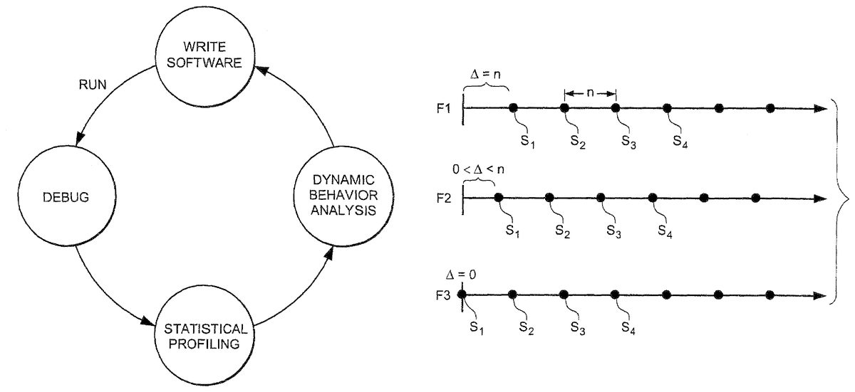
FIG. 2depicts a sequence of steps in the process of developing software using such statistical profiler analysis. A software developer writes a program, which is executed in a computer processor. In order to look for errors in the software program (an activity referred to as “debugging”) or for other purposes, the execution of the software code is effected using statistical profiling. The results of the statistical profiling offer a picture of the dynamic behavior of the program during its execution. Based on this analysis, the developer is in better position to change the original software code so that its dynamic operation is optimized. This process can be performed iteratively as shown.

A. Efficient Statistical Profiling By Varying the Distribution of the Samples within a Frame

Typically, a media processing system, such as a video game console or a real-time simulation system may form an image or picture on a display by generating the display one line or frame at a time. For example, in a raster scan display, the instantaneous brightness at a particular physical point on the display is represented by the amplitude of the electrical signal. The scanning circuit retraces to the left edge of the display and then starts scanning the next line. Starting at the top of the display, all of the lines on the display are scanned in this way. One complete set of lines makes a picture of image. This is referred to as a frame. Once the first complete picture is scanned, the scanning circuit retraces to the top of the display and starts scanning the next frame. In case of video signals, this process is repeated so fast that the human eye blends the succeeding frames together and displayed images are perceived to have a continuous motion.

The media processing system may display the media information in several display or scan modes. Examples of scan modes include interlaced and non-interlaced (progressive) modes. Such modes are related to different scanning techniques. Television signals and compatible displays are typically interlaced, and computer signals and compatible displays are typically non-interlaced.

In interlaced scanning, a frame representing a picture is split into two separate fields. One field may include odd lines of the picture and the other field may include even lines of the picture. The two fields constitute a frame. A picture formed by interlaced scanning is drawn on the screen in two passes, first by scanning the horizontal lines in the first field, and then scanning (or interlacing) the horizontal lines in the second field in-between the first set of lines. Interlacing field1and field2at 60 fields per second yields an effective 30 frames per second frame rate.

In non-interlaced scanning, the picture is formed on the display by scanning all of the horizontal lines of the picture in one pass from the top to the bottom. This is sometimes referred to as “progressive scanning’. Unlike interlaced scanning, progressive scanning involves complete frames including both odd and even lines, in other words, each scan displays an entire frame. For example, in progressive scanning, a frame rate of 60 frames per second causes 60 frames to be formed on the display, in contrast to interlaced scanning, where a field rate of 60 fields per second causes only 30 frames per second to form on the display.

Whatever the frame rate is, the exemplary illustrative non-limiting implementation described herein generates well spaced samples that vary from frame to frame. In order to achieve this, the exemplary illustrative non-limiting implementation uses a hybrid random sample distribution, wherein a fixed sampling rate is used, but the first sampling point in each frame has a random offset from the beginning of the frame.FIG. 3depicts such a sampling method. Three successive exemplary frames F1, F2and F3are shown. Sampling occurs during times S1, S2, S3. . . SN. The number N of sampling points can be any number such as thousands, or millions. The interval between the sampling points may be constant. The number of samples per frame may be different, but the spacing between the samples can be the same. In one exemplary illustrative non-limiting implementation, the first sampling point S1of a particular frame is taken Δ sec after the beginning of the frame, where Δ is a random number. The random offset is in the range of [0, n], where n is the time between fixed samples. For example, if the fixed sampling rate is 1,000 times per second, then the time between samples is 0.001 seconds. Therefore, in this example, the random offset is in the range [0, 0.001]. InFIG. 3, the offset is the largest in the top frame F1, the lowest in the bottom frame F3, and somewhere in between in frame F2.

The exemplary illustrative fixed sampling rate ensures that samples within a frame are well distributed. In addition, significant variation in the random offsets from frame to frame results in a good sampling distribution from frame to frame. In one exemplary illustrative non-limiting implementation, to ensure great variation of the sampling distribution from frame to frame, the range for the offset is varied for each frame, and it may be based on the ranges used in previous frames. In other words, the goal is to generate random numbers for each offset based on ranges that do not lie too close to previous values. For example, if the whole range of possible offsets is [0, 1], and the last two frame offsets were 0.13 and 0.96, then the range for the next offset might be [0.23, 0.86]. This exemplary implementation satisfies the requirement that consecutive offsets cause the sampling to vary significantly from frame to frame. Non-random variable offsets could be used if desired, or various techniques could be used for determining different offsets for different frames to provide representative sample times.

The above exemplary illustrative hybrid random sampling rate allows for samples within an individual frame or a small group of frames to be analyzed with a high degree of confidence, because they represent a statistically accurate view of the true program behavior.

B. Efficient Statistical Profiling by Efficiently Representing the Form of the Samples

Statistical profiling may generate a great amount of data due to the sampling of the executing code. This represents a challenge to efficiently storing the accumulated data. The exemplary illustrative non-limiting technology herein addresses this challenge by effectively manipulating two aspects of the profile data: the individual samples, both cumulatively and individually, and a resulting call graph structure of the program being profiled.

First, the treatment of a single profile sample in a statistical sampling profiler is examined. When a statistical sampling profiler takes a sample, it temporarily interrupts the program execution and records the call stack. This stack comprises a series of addresses, which represent positions within various functions running during the execution of the program. For example, as shown inFIG. 4, the call stack may contain the functions: “Main”, “CalculateCollisions”, and “DistanceTest” with the respective addresses: “0x1038”, “0x3324”, and “0x4420”. This indicates that the function “Main” called the function “CalculateCollisions”, which in turn called the function “DistanceTest”. The composition of the call stack further indicates that the program execution was ultimately stopped/sampled inside the function “DistanceTest”. The corresponding addresses indicate where in memory the program instructions are stored for the currently executing instructions at each moment and for each function level.

Generally, each function is composed of many individual instructions (i.e., steps that produce the desired result at the end), with all the instructions in a function stored at sequential series of addresses in the memory. For example, as shown inFIG. 5, the function “DistanceTest” has its first instruction located at the 0x4000 address, and its last instruction before 0x5000, with corresponding range of addresses for the other functions. When the exemplary illustrative profiler captured a sample in the above example, the current execution at that point was in the middle of the function “DistanceTest”, namely at the 0x4420 address. For the profiler to determine which function contains the instruction address 0x4420, it consults the list of all function start addresses and function sizes. This list can be generated by the compiler when the program is compiled. However, for an embedded device, the list of function addresses and sizes is often large in terms of memory, and may reside on the PC side (where the program was compiled). Thus it may be transmitted to the embedded device before the profiling process may begin.

An exemplary illustrative non-limiting implementation involves transmitting the list of function addresses to the embedded device before profiling begins. Moreover, to promote efficiency, only the function start addresses need to be sent. Not all function addresses are necessarily sent to the embedded device nor their sizes (since the size of each function can be inferred from this truncated data). Given an arbitrary address inside a function, and using only the list of function start addresses, it is possible to find the start address of a function for an arbitrary address by performing a binary search on the list. For example, if the function start addresses were (0x1000, 0x2000, 0x3000, 0x4000, 0x5000, 0x6000) and the arbitrary address in the sample was 0x4420, then a binary search would find the corresponding start address 0x4000 in two steps, or generally in log N steps, where N is the number of addresses in the list. Other comparable methods such as a hash table could also be used.

Typically, in a statistical sampling profiler, the call stack data is simply collected and stored without any additional processing. In the case where the embedded device has only a small amount of memory available, there may be a strict memory requirement for storing the profile data. The solution is to process each address taken during the profiling to discover the true start address of the function that contains the address. If the sampled data is transformed to only contain start addresses, then the sample data can be sorted and accumulated while at the same time the amount of stored data can be drastically reduced. For example, if 1,000,000 samples are taken with an average call stack depth (i.e., number of addresses) of 14, then profiling in a traditional profiling system, there are 14,000,000 addresses to store. However, if each function address is transformed into its start address, then the addresses can be sorted and accumulated in a tree form. SeeFIGS. 7A and 7Bfor exemplary binary call graph trees. If the call graph tree contains 1,000 functions, each with a corresponding start address, then there are only 1,000 addresses with 1,000 corresponding function counts (representing how many times that function is the tree was sampled), and 2,000 internal tree pointers, resulting in approximately 4,000 stored data items. Comparing this number to the total number of data items stored in a traditional profiler (and assuming that all addresses, counts and pointers are individually the same size in bytes), it is seen that the exemplary illustrative non-limiting data structure implementation is 3,500 times smaller than the raw data.

To further illustrate how the transformation technique may affect the call graph resulting from the samples taken during the profiling, the following example is given, where five raw profile samples are taken during the profiling process:

Sample 1:0x1038,0x3234,0x4420Sample 2:0x1038,0x3234,0x4868Sample 3:0x1038,0x3438Sample 4:0x1330,0x2874,0x5920Sample 5:0x1574,0x4760

After determining the start address for each address, the profile samples become:

Sample 1:0x1000,0x3000,0x4000Sample 2:0x1000,0x3000,0x4000Sample 3:0x1000,0x3000Sample 4:0x1000,0x2000,0x5000Sample 5:0x1000,0x4000

This data can be compactly represented in the following tree form:

0x1000, count 0|−0x3000, count 1| || −0x4000,  count 2|−0x2000, count 0| || −0x5000,  count 1|−0x4000, count 1

The count number at each node can be incremented each time the function was called, corresponding to the number of samples recording the call of that function. For example, during the time interval corresponding to five samples given above, the sequence of functions having corresponding starting addresses 0x1000, 0x3000, 0x4000 was called twice.

In a “first child-next sibling” binary tree form, where each node may have two links, one leading to a “first child” node and one leading to a “next sibling” node, which is the next node at the same level, the tree would have the following representation (X denotes a NULL value):

Index 0:(0x1000,First Child = 1,Next Sibling = X)Index 1:(0x3000,First Child = 2,Next Sibling = 3)Index 2:(0x4000,First Child = X,Next Sibling = X)Index 3:(0x2000,First Child = 4,Next Sibling = 5)Index 4:(0x5000,First Child = X,Next Sibling = X)Index 5:(0x4000,First Child = X,Next Sibling = X)

The above can be stored as an array of triples:

[(0x1000,1,X), (0x3000,2,3), (0x4000,X,X), (0x2000,4,5), (0x5000,X,X), (0x4000,X,X)]

The frequency count data is stored as a horizontal array, with each index correlated to the same index in the binary tree:

[0, 1, 2, 0, 1, 1]

The above process can be described in reference toFIG. 6, wherein in the top portion100, frames “A’, “B”, “C”, etc. depict a sequence of nodes in the tree, i.e., starting addresses of functions, e.g., 0x1000, 0x2000, etc. Each frame corresponding to a function also includes a sub-frame corresponding to the “child” node and possibly a “next sibling” node resulting from the specific node. Based on the sequence of the various functions called by the program, a parallel frequency counter array110is provided that records the number of times each specific function in the top list is called.

In the exemplary illustrative non-limiting implementation, the call graph tree is typically built up relatively quickly with a small amount of sample data, whereas the frequency count array is continuously updated with each sample. Therefore, it may be advantageous and more cache and memory efficient to store the accumulated frequency count array separately from the call graph tree.

One consequence of accumulating profile samples into a call graph tree, is that individual frames (samples during a particular simulation loop) are lost as they are collapsed into the data over all the frames. Another implementation of this technique, at the cost of additional memory, preserves the individual sample data by storing only a pointer to the leaf node in the call graph tree for each sample. Only the leaf is needed, since the parents (or calling functions) are explicitly represented in the tree. In this way, additional memory of recording an entire call stack for each sample can be avoided.

For example, if 1,000,000 samples are taken with an average stack depth of 14, the traditional implementation would store 14,000,000 addresses. If each sample taken augments the call graph tree, then as discussed in the earlier example, it would result in 3,000 stored data items (i.e., 1,000 function addresses and 2,000 tree pointers). In addition, if each sample was recorded with a pointer to some node in the call graph tree, then there would be an 1,000,000 pointers. If we assume that each stored item is 4 bytes long, then at least some traditional methods store 56,000,000 bytes as compared to the exemplary illustrative non-limiting call graph implementation with pointers, which stores 4,012,000 bytes, 14 times smaller.

Given the previous example of profile samples and a corresponding call graph tree, the five stored samples (converted to pointers that refer to the indices of the call graph binary tree) would have the following representation:

Sample 1: 2

Sample 2: 2

Sample 3: 1

Sample 4: 4

Sample 5: 5

As an array of samples, it would appear as:

[2, 2, 1, 4, 5]

If the embedded device has enough memory to record all raw profile samples, the disclosed method could be applied as a post-process, for making the data still more efficient to transmit from the embedded device to the connected PC.

Efficient representation of statistical profile samples is highly desirable when profiling on an embedded device, which lacks sufficient memory and/or adequate communication speed with a connected PC. By efficiently representing the raw sample data and the corresponding call graph data structure, millions of samples can be stored using magnitudes of less memory compared to traditional statistical profiling systems. Either technique of utilizing the frequency count array or the storing individual samples pointing back to the call graph reduces the memory overhead, facilitates the storage capability of the device and increases the communication times with a connected PC.

While the technology herein has been described in connection with exemplary illustrative non-limiting embodiments, the invention is not to be limited by the disclosure. The invention is intended to be defined by the claims and to cover all corresponding and equivalent arrangements whether or not specifically disclosed herein.